Seven Ways to Create a Storymap
Tony Hirst - August 25, 2014 in Data Journalism, Data Stories, HowTo, Storytelling
If you have a story that unfolds across several places over a period of time, storymaps can provide an engaging interactive medium with which to tell the story. This post reviews some examples of how interactive map legends can be used to annotate a story, and then rounds up seven tools that provide a great way to get started creating your own storymaps.
Interactive Map Legends
The New York Times interactives team regularly come up with beautiful ways to support digital storytelling. The following three examples all mahe use of floating interactive map legends to show you the current location a story relates to as they relate a journey based story.
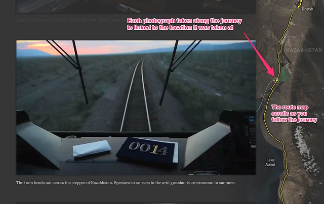
Riding the Silk Road, from July 2013, is a pictorial review featuring photographs captured from a railway journey that follows the route of the Silk Road. The route is traced out in the map on the left hand side as you scroll down through the photos. Each image is linked to a placemark on the route to show where it was taken.
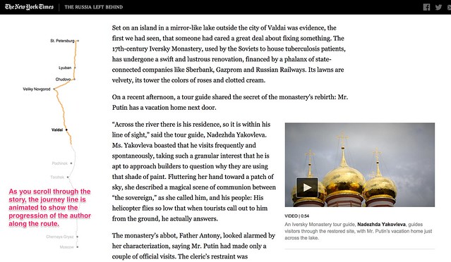
The Russia Left Behind tells the story of a 12 hour drive from St. Petersburg to Moscow. Primarily a textual narrative, with rich photography and video clips to illustrate the story, an animated map legend traces out the route as you read through the story of the journey. Once again, the animated journey line gives you a sense of moving through the landscape as you scroll through the story.
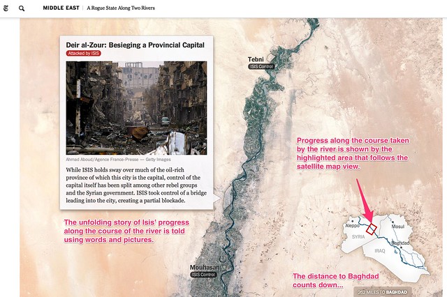
A Rogue State Along Two Rivers, from July 2014, describes the progress made by Isis forces along the Tigris and Euphrates Rivers is shown using two maps. Each plots the course of one of the rivers and uses place linked words and photos to tell the story of the Isis manoeuvres along each of the river ways. An interactive map legend shows where exactly along the river the current map view relates to, providing a wider geographical context to the local view shown by the more detailed map.
All three of these approaches help give the reader a sense of motion though the journey traversed that leads the narrator being in the places described at different geographical storypoints described or alluded to in the written text. The unfolding of the map helps give the reader the sense that a journey must be taken to get from one location to another and the map view – and the map scale – help the reader get a sense of this journey both in terms of the physical, geographical distance it relates to and also, by implication, the time that must have been expended on making the journey.
A Cartographic Narrative
Slave Revolt in Jamaica, 1760-1761, a cartographic narrative, a collaboration between Axis Maps and Harvard University’s Vincent Brown, describes itself as an animated thematic map that narrates the spatial history of the greatest slave insurrection in the eighteenth century British Empire. When played automatically, a sequence of timeline associated maps are played through, each one separately animated to illustrate the supporting text for that particular map view. The source code is available here.
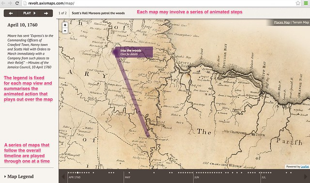
This form of narrative is in many ways akin to a free running, or user-stepped, animated presentation. As a visual form, it also resembles the pre-produced linear cut scenes that are used to set the scene or drive the narrative in an interactive computer game.
Creating you own storymaps
The New York Times storymaps use animated map legends to give the reader the sense of going on a journey by tracing out the route being taken as the story unfolds. The third example, A Rogue State Along Two Rivers also makes use of a satellite map as the background to the story, which at it’s heart is nothing more than a set of image markers placed on to an an interactive map that has been oriented and constrained so that you can only scroll down. Even though the maps scrolls down the page, the inset legend shows the route being taken may not be a North-South one at all.
The linear, downward scroll mechanic helps the reader feel as if they are reading down through a story – control is very definitely in the hands of the author. This is perhaps one of the defining features of the story map idea – the author is in control of unraveling the story in a linear way, although the location of the story may change. The use of the map helps orientate the reader as to where the scenes being described in the current part of the story relate to, particularly any imagery.
Recently, several tools and Javascript code libraries have been made available from a variety of sources that make it easy to create your own story maps within which you can tell a geographically evolving story using linked images, or text, or both.
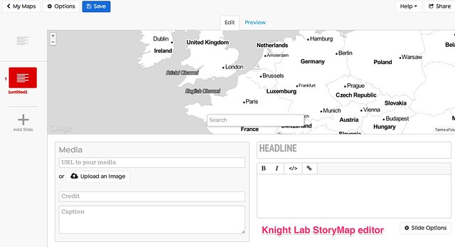
Knight Lab StoryMap JS
The Knight Lab StoryMap JS tool provides a simple editor synched to a Google Drive editor that allows you to create a storymap as a sequence of presentation slides that each describe a map location, some header text, some explanatory text and an optional media asset such as an image or embedded video. Clicking between slides animates the map from one location to the next, showing a line between consecutive points to make explicit the linkstep between them. The story is described using a custom JSON data format saved to the linked Google Drive account.
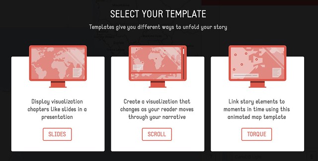
CartoDB Odyssey.js
Odyssey.js provides a templated editing environment that supports the creation of three types of storymap: a slide based view, where each slide displays a location, explanatory text (written using markdown) and optional media assets; a scroll based view, where the user scrolls down through a stroy and different sections of the story trigger the display of a particular location in a map view fixed at the top of the screen; and a torque view which supports the display and playback of animated data views over a fixed map view.
A simple editor – the Odyssey sandbox – allows you to script the storymap using a combination of markdown and map commands. Storymaps can be published by saving them to a central githib repository, or downloaded as an HTML file that defines the storymap, bundled within a zip file that contains any other necessary CSS and Javascript files.
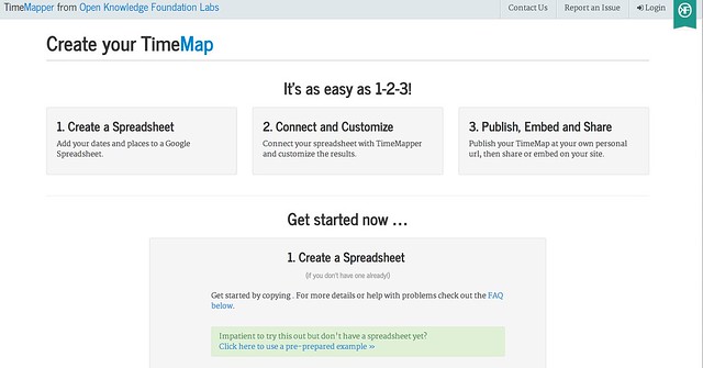
Open Knowledge TimeMapper
TimeMapper is an Open Knowledge Labs project that allows you to describe location points, dates, and descriptive text in a Google spreadsheet and then render the data using linked map and timeline widgets.
JourneyMap (featuring waypoints.js
JourneyMap is a simple demonstration by Keir Clarke that shows how to use the waypoints.js Javascript library to produce a simple web page containing a scrollable text area that can be used to trigger the display of markers (that is, waypoints) on a map.
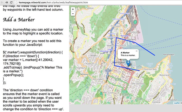
[waypoints.js on Githhub; JourneyMap src]
Google Earth TourBuilder
Google Earth TourBuilder is a tool for building interactive 3D Google Earth Tours using a Google Earth browser plugin. Tours are saved (as KML files?) to a Google Drive account.
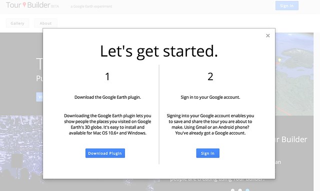
[Note: Google Earth browser plugin required.]
ESRI/ArcGIS Story Maps
ESRI/ArcGIS Story Maps are created using an online ArcGIS account and come in three type with a range of flavours for each type: “sequential, place-based narratives” (map tours), that provide either an image carousel (map tour) that allows you to step through a sequence of images that are displayed separately alongside a map showing a corresponding location or a scrollable text (map journal) with linked location markers (the display of half page images rather than maps can also be triggered from the text); curated points-of-interest lists that provide a palette of images, each member of which can be associated with a map marker and detailed information viewed via a pop-up (shortlist), a numerically sequence list that displays map location and large associated images (countdown list), and a playlist that lets you select items from a list and display pop up infoboxes associated with map markers; or map comparisons provided either as simple tabbed views that allow you to describe separate maps, each with its own sidebar description, across a series of tabs, with separate map views and descriptions contained within an accordion view, and swipe maps that allow you to put one map on top of another and then move a sliding window bar across them to show either the top layer or the lower layer. A variant of the swipe map – the spyglass view alternatively displays one layer but lets you use a movable “spyglass” to look at corresponding areas of the other layer.

[Code on github: map-tour (carousel) and map journal; shortlist (image palette), countdown (numbered list), playlist; tabbed views, accordion map and swipe maps]
Leaflet.js Playback
Leaflet.js Playback is a leaflet.js plugin that allows you to play back a time stamped geojson file, such as a GPS log file.
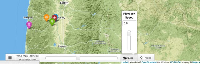
[Code on Github]
Summary
The above examples describe a wide range of geographical and geotemporal storytelling models, often based around quite simple data files containing information about individual events. Many of the tools make a strong use of image files as pat of the display.
it may be interesting to complete a more detailed review that describes the exact data models used by each of the techniques, with a view to identifying a generic data model that could be used by each of the different models, or transformed into the distinct data representations supported by each of the separate tools.
UPDATE 29/8/14: via the Google Maps Mania blog some examples of storymaps made with MapboxGL, embedded within longer form texts: detailed Satellite views, and from the Guardian: The impact of migrants on Falfurrias [scroll down]. Keir Clarke also put together this demo: London Olympic Park.
UPDATE 31/8/14: via @ThomasG77, Open Streetmap’s uMap tool (about uMap) for creating map layers, which includes a slideshow mode that can be used to create simple storymaps. uMap also provides a way of adding a layer to map from a KML or geojson file hosted elsewhere on the web (example).
![]()