You are browsing the archive for SQL.

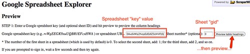
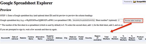
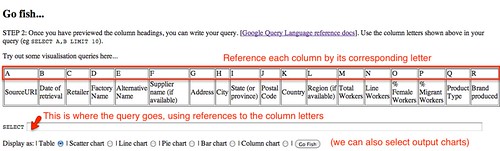
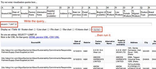
SQL: The Prequel (Excel vs. Databases)

- November 7, 2013 in HowTo, Spreadsheets, SQL

Table à encrer les rouleaux d’imprimerie

Image credit: Frédéric Bisson

School of Data is re-publishing Noah Veltman‘s Learning Lunches, a series of tutorials that demystify technical subjects relevant to the data journalism newsroom.

This first Learning Lunch is about the database query language SQL and how it compares to Excel.

What Excel is good at

Excel gets a bad rap. It’s a very flexible, powerful piece of software that’s good at a lot of things.

  • It’s easy to browse data.
  • It’s easy to manually enter and edit data.
  • It’s easy to share copies of files.
  • You have fine control over visual presentation.
  • It has a very flexible structure. Every cell is a unique snowflake.
  • It integrates with other popular office software.
  • Formulas make it a living document.
  • It has a built-in suite of helpers for charts, comments, spellchecking, etc.
  • It’s relatively easy to learn.

What Excel is bad at

Unfortunately Excel also has its limits. It’s pretty bad at some other things.

  • It lacks data integrity. Because every cell is a unique snowflake, things can get very inconsistent. What you see doesn’t necessarily represent the underlying data. A number is not necessarily a number. Data is not necessarily data. Excel tries to make educated guesses about you want, and sometimes it’s wrong.
  • It’s not very good for working with multiple datasets in combination.
  • It’s not very good for answering detailed questions with your data.
  • It doesn’t scale. As the amount of data increases, performance suffers, and the visual interface becomes a liability instead of a benefit. It also has fixed limits on how big a spreadsheet and its cells can be.
  • Collaborating is hard. It’s hard to control versions and have a “master” set of data, especially when many people are working on the same project (Google Spreadsheets fix some of this).

Enter relational databases

What is a relational database? We could get very picky about terminology, but let’s not. Broadly speaking, it consists of a “server” that stores all your data (think of a huge library) and a mechanism for querying it (think of a reference librarian).

The querying is where SQL comes in, emphasis on the Q. SQL stands for Structured Query Language, and it is a syntax for requesting things from the database. It’s the language the reference librarian speaks. More on this later.

The “relational” part is a hint that these databases care about relationships between data. And yes, there are non-relational databases, but let’s keep this simple. We’re all friends here.

The database mantra

Everything in its proper place.

A database encourages you to store things logically. Sometimes it forces you to.

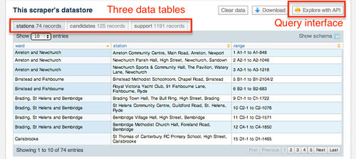
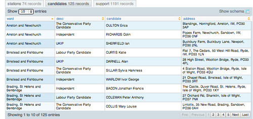
Every database consists of tables. Think of a table like a single worksheet in an Excel file, except with more ground rules. A database table consists of columns and rows.

Columns

Every column is given a name (like ‘Address’) and a defined column type (like ‘Integer,’ ‘Date’, ‘Date+Time’, or ‘Text’). You have to pick a column type, and it stays the same for every row. The database will coerce all the data you put in to that type. This sounds annoying but is very helpful. If you try to put the wrong kind of data in a column, it will get upset. This tells you that there’s a problem with your data, your understanding of the data, or both. Excel would just let you continue being wrong until it comes back to bite you.

You can also specify helpful things like…
… whether a column can have duplicate values.
… whether a column can be empty.
… the default value for a column if you don’t specify one.

Columns define the structure of your data.

Rows

Rows are the actual data in the table. Once you establish the column structure, you can add in as many rows as you like.

Every row has a value for every column. Excel is a visual canvas and will allow you to create any intricate quilt of irregular and merged cells you’d like. You can make Tetris shapes and put a legend in the corner and footnotes at the bottom, all sharing the same cells.

This won’t fly with a database. A database table expects an actual grid. It’s OK for cells to be empty, but to a computer intentionally empty is not the same as nonexistent.

Multiple tables, joins, and keys

More on this later, but part of putting everything in its proper place means making it easy to break up your data into several tables for different data categories and work with them as a set.

Let data be data.

A database focuses only on the data layer of things and ignores visual presentation. Colors, fonts, borders, date formatting, and number formatting basically don’t exist. What you see is mostly what you get. That’s good news and bad news: it means that a database is usually really good at what it does do, but it also often needs to be paired with other things in order to create a final product, like a chart or a web page. A database is designed to plug in to other things. This extra step is one of the things that turns a lot of people off to databases.

By being really good at data storage and processing and not at other things, databases are extremely scaleable. 1 million rows of data? 10 million? No problem. For newsroom purposes, there’s virtually no upper limit to how much data you can store or how complicated you can make your queries.

Databases & the web

Databases are great for preliminary analysis, exploration, and data cleaning. But they’re even better for connecting to something else once you know what you want to do with the data. Virtually every web application is powered by databases like this. When you log in somewhere, it’s checking your username and password against a database. When you go to IMDB and click on a movie, it’s looking up a database. Twitter, Facebook, Gmail, it’s databases all the way down.

When it comes to news features, a database usually gets involved when the amount of data is large or it is expected to change over time. Rather than having a static JSON file with your data, you keep a database and you write an app that queries the database for the current data. Then, when the data changes, all you have to do is update the database and the changes will be reflected in the app. For one-off apps where the data is not going to change and the amount is small, a database is usually overkill, although you may still use one in the early stages to generate a data file of some sort.

If you’re using an API to feed current data into an app instead, you’re still using a database, you’re just letting someone else host it for you. This is much easier, but also poses risks because you access the data at their pleasure.

Potential semantic quibble: sometimes an app isn’t directly accessing a database to fetch information. Sometimes it’s accessing cached files instead, but those cached files are generated automatically based on what’s in the database. Tomato, Tomahto.

So when should I use a database instead of Excel?

Excel and databases are good for very different things. Neither is per se good or bad. A rule of thumb: you should strongly consider using a database for a project to the extent that the following are true:

  • You have a lot of data.
  • Your data is messy or complex.
  • You want to power something else with your data.
  • Other people need to work with the same data.

OK, I’m intrigued. How do I get started?

Because databases have a learning curve, it makes sense not to dive in too deep right away. Start off using it only in cases where the advantage is especially strong and your needs are pretty simple. As your comfort level increases, you’ll increasingly look towards databases to get what you want faster.

Option 1: SQLite

SQLite is a good way to get started. You can install the “SQLite Manager” add-on for Firefox and do everything within the browser.

A SQL tutorial based on SQLite: https://github.com/tthibo/SQL-Tutorial

Option 2: Microsoft Access

Microsoft Access runs on SQL and presents a more traditional desktop software interface. Depending on who you ask, it’s either a helpful tool or just makes things more confusing. I wouldn’t personally recommend it, but your mileage may vary.

Option 3: Set up a shared web hosting account

You can set up a shared web hosting account as a sandbox to play with this. This can cost as little as £20 a year. These accounts typically come with an interface to let you create, edit, and interact with databases without writing any SQL. They also give you a place to play around with any other web-related skills you’re interested in and share the results with others!

A Small Orange (a good, cheap hosting option): http://asmallorange.com/

Option 4: Install MySQL or PostgreSQL on your computer

You can install MAMP on a Mac or WAMP on a Windows PC. This will install MySQL as well as a great web-based interface called phpMyAdmin (http://www.phpmyadmin.net). Once you have MySQL installed, you have lots of additional options for free software to serve as a browser/editor for your SQL databases. If you prefer you can install PostgreSQL instead, a slightly different database flavor (there are many different flavors of database but MySQL and PostgreSQL are two popular ones with lots of documentation, don’t overthink it for now).


Appendix: querying for fun and profit

Much of the power of relational databases comes from SQL, a very flexible language for asking a database questions or giving it orders. The learning curve is steeper than Excel, but once you get the hang of it you can quickly answer almost any question about your data. Let’s go through some brief examples of how a desired action looks in SQL.

The basic building blocks of SQL are four verbs: SELECT (look up something), UPDATE (change some existing rows), INSERT (add some new rows), DELETE (delete some rows). There are many other verbs but you will use these the most, especially SELECT.

Let’s imagine a table called athletes of Olympic athletes with six columns:

name
country
birthdate
height
weight
gender

When creating our table, we might also specify things like “country can be empty” or “gender must be either M or F.”

Query 1: Get a list of all the athletes in alphabetical order. This will show you the entire table, sorted by name from A-Z.

SELECT
*
FROM athletes
ORDER BY name ASC

Query 2: Get a list of all the athletes on Team GB. This will show you only the rows for British athletes. You didn’t specify how to sort it, so you can’t count on it coming back in the order you want.

SELECT
*
FROM athletes
WHERE country = 'Great Britain'

Query 3: What country is the heaviest on average? This will take all the rows and put them into groups by country. It will show you a list of country names and the average weight for each group.

SELECT
country,AVG(WEIGHT)
FROM athletes
GROUP BY country

Query 4: What birth month produces the most Olympic athletes? Maybe you want to test an astrological theory about Leos being great athletes. This will show you how many Olympic athletes were born in each month.

SELECT
MONTHNAME(birthdate),COUNT(*)
FROM athletes
GROUP BY MONTHNAME(birthdate)

Query 5: Add a new athlete to the table. To insert a row, you specify the columns you’re adding (because you don’t necessarily need to add all of them every time), and the value for each.

INSERT
INTO athletes
(name,country,height,weight,gender)
VALUES ('Andrew Leimdorfer','Great Britain',180,74.8,'M')

Query 6: Get all male athletes in order of height:weight ratio. Maybe you would notice something strange about Canadian sprinter Ian Warner.

SELECT
*
FROM athletes
WHERE gender = 'M'
ORDER BY height/weight ASC

Query 7: If you got your data from london2012.com, you would think 5′ 7″ Ian Warner was 160 kg, because his weight was probably entered in lbs instead. Let’s fix that by UPDATEing his row.

UPDATE
athletes
SET weight = weight/2.2
WHERE NAME = 'Ian Warner'

Query 8: Delete all the American and Canadian athletes, those jerks.

DELETE
FROM athletes
WHERE country = 'United States of America' OR country = 'Canada';

Once you look at enough queries you’ll see that a query is like a sentence with a grammar. It has a “verb” (what kind of action do I want?), an “object” (what tables do I want to do the action to?), and optional “adverbs” (how specifically do I want to do the action?). The “adverbs” include details like “sort by this column” and “only do this for certain rows.”

Bonus Level: multiple tables and a brief taste of JOINs

You probably have a lot more data than just athletes. For each country, you might also have its flag, its population, and its capital city. You also have all the Olympic events, which athletes participated in them, which venues they were at, which sport category they belong to. For each event, you also end up with results: who got which medals, and in some cases what the finishing times/scores were.

The typical Excel approach to this is one of two forms of madness: either you have a bunch of spreadsheets and painstakingly cross-reference them, or you have one mega-spreadsheet with every column (government data sources love mega-spreadsheets).

You might have a spreadsheet where each row is an athlete, and then you have a long list of columns including lots of redundant and awkwardly-stored information, like:

name, country, birthdate, height, weight, gender, country_population, country_flag_url, country_gdp, event1, event1_date, event1_result, event2_date, event2_result, event3_date, event3_result, event4_date, event4_result, number_of_medals

This mega-spreadsheet approach has all kinds of weaknesses:

  • You lose the benefit of visually browsing the information once a table gets this big. It’s a mess.
  • This structure is very inflexible. The law of mega-spreadsheets states that once you arbitrarily define n columns as the maximum number of instances a row could need, something will need n+1.
  • It has no sense of relationships. Athletes are one atomic unit here, but there are others. You have countries, you have events (which belong to sports), you have results (which belong to events), you have athletes (which compete in events, have results in those events, and almost always belong to countries). These relationships will probably be the basis for lots of interesting stories in your data, and the mega-spreadsheet does a poor job of accounting for them.
  • Analysis is difficult. How do you find all the athletes in the men’s 100m dash? Some of them might have their time in event1_result, some of them might have it in event2_result. Have fun with those nested IF() statements! And if any of this data is manually entered, there’s a good chance you’ll get textual inconsistencies between things like “Men’s 100m,” “Men’s 100 meter,” and “100m.”

SQL lets you keep these things in a bunch of separate tables but use logical connections between them to smoothly treat them as one big set of data. To combine tables like this, you use what are called JOINs. In a single sentence: a JOIN takes two tables and overlaps them to connect rows from each table into a single row. JOINs are beyond the scope of this primer, but they are one of the things that make databases great, so a brief example is in order.

You might create a table for athletes with basic info like height & weight, a table for events with details about where and when it takes place and the current world record, a table for countries with information about each country, and a table for results where each row contains an athlete, an event, their result, and what medal they earned (if any). Then you use joins to temporarily combine multiple tables in a query.

Who won gold medals today?

SELECT
athletes.name, athletes.country, event.name
FROM athletes, results, events
WHERE athletes.id = results.athlete_id AND event.id = results.event_id
AND event.date = DATE(NOW()) AND results.medal = 'Gold'

How many medals does each country have?

SELECT
countries.name, COUNT(*)
FROM athletes, countries, results, events
WHERE athletes.id = results.athlete_id AND event.id = results.event_id AND athletes.country_id = countries.id
AND results.medal IN ('Gold','Silver','Bronze')
GROUP BY countries.id

Flattr this!

Asking Questions of Data – Garment Factories Data Expedition

- May 24, 2013 in Spreadsheets, SQL

As preparation for the upcoming data expedition on Mapping the garment factories this weekend, several intrepid explorers have been collating data from brand supplier lists that identify the location of over 3,000 factories to date.

The data is being published via a Google Spreadsheet, which means we can also treat it as a database, asking database like queries either within the spreadsheet itself, or via a webservice.

The School of Data blogpost Asking Questions of Data – Some Simple One-Liners introduced the idea of using SQL – the Structured Query Language – to ask questions of a dataset contained in a small database populated with data that had been “liberated” using Scraperwiki. The query language that Google Spreadsheets supports is rather like a cut down version of SQL, so it can be a good place to start learning how to write such queries.

The query language allows us to select just those databasespreadsheet rows where a particular column contains a particular value, such as rows relating to factories located in a particular country or supplying a particular brand. We can also create more complex queries, for example identifying factories located in a particular country that supply a particular brand. We can also generate summary reports, such as listing all the brands identified, or counting all the factories within each city in a particular country.

I’ve posted an informal, minimal interface to the query API here: Google Spreadsheet Query Interface (feel free to clone the view and improve on it!)

spreadsheet explorer config

Paste in the spreadsheet key value, which for the garment factory spreadsheet is 0AvdkMlz2NopEdEdIZ3d4VlFJQ0NkazhrWGFQdXZQMkE, along with the sheet’s “gid” value – 0 for the sheet we want. If you click on the Preview button, we can see the column headings:

spreadsheet query preview headings

We can now start to ask questions of the data, building up a query around the different spreadsheet columns. For convenience (?!), we can use the letters that identify each column in the spreadsheet to help build up out query.

google spreadsheet query form

Let’s start with a simple query that shows all the columns (*) for the first 10 rows (LIMIT 10)

We would write the query out in full as:

SELECT * LIMIT 10

but the form handles the initial SELECT statement for us, so all we need to write is:

* LIMIT 10

Run the query by clicking ion the “Go Fish” button, and the results should appear in a table.

run a query

Note that you can sort the rows in the table by clicking on the appropriate column header. The query form also allows you to preview queries using a variety of charts, although for these to work you will need to make sure you select appropriate columns as we’ll see later.

As well as generating a tabular (or chart based) view of the results, the running the query also generates couple of links, one to an HTML table view of the results, one to a CSV formatted version of the data.

csv and html output links

If you look at the web addresses/URLs that are generated for these links, you may notice they are “hackable” (Hunting for Data – Learning How to Read and Write Web Addresses, aka URLs ).

Knowing that the spreadsheet provides us with database functionality allows us to do two different things. Firstly, we can run queries on the data to generate subsets of it, for example as CSV files, that we can load into other tools for analysis purposes. Secondly, we can generate reports on the data that may themselves be informative. Let’s look at each in turn.

Generating subsets of data

In the simplest case, there are two main ways we can generate subsets of data. If you look at the column headings, you will notice that we have separate columns for different aspects of the dataset, such as the factory name, the company it supplies, the country or city it is based in, and so on. Not all the separate factory results (that is, the separate rows of data) have data in each column, which is something we may need to be aware of!)

In some reports, we may not want to see all the columns, so instead we can select just those columns we want:

SELECT C, D, K,R LIMIT 10

simple select

To see all the results, remove the LIMIT 10 part of the query.

We can also rearrange the order of columns by changing the order in which they appear in the query:

SELECT D, C, K, R LIMIT 10

reorder columns

The second form of subsetting we can do is to limit the rows that are displayed dependent on whether they contain a particular value, or more specifically, when the value of a cell from that row contains a particular value in a particular column.

So for example, here’s a glimpse of some of the factories that are located in India:

SELECT D, C, K, R WHERE K='INDIA' LIMIT 10

some Indian factories

To see all the countries that are referenced, some query languages allow us to use a DISTINCT search limit. The Google Query Language does not support the DISTINCT operator, but we can find another way of getting all the unique values contained within a column using the GROUP BY operator. GROUP BY says “find all the elements in a column that have the same value, and for each of these groups, do something with it”. The something-we-can do might simply be to count the number of the rows in the group, we which can do as follows (COUNTing on any column other than the GROUP BY column(s) will do).

SELECT K, COUNT(A) GROUP BY K LIMIT 10

finesse distinct

See if you can work out how to find the different Retailers represented in the dataset. Can you also see how to find the different retailers represented in a particular country?

One of the things you may notice from the above result is that “ARGENTINA” and “Argentina” are not the same, and neither are ‘BANGLADESH’ and ‘Bangladesh’…

If we wanted to search for all the suppliers listed in that country, we could do a couple of things:

  • SELECT C, K WHERE K='BANGLADESH' OR K='Bangladesh' – in this case, we accepts results where the Country column value for a given row is either “BANGLADESH” or it is “Bangladesh”.

  • SELECT C, K WHERE UPPER(K)='BANGLADESH' – in this case, we set the cell value to its uppercase equivalent, and then test to see if it matches ‘BANGLADESH’

In a certain sense, the latter query style is applying an element of data cleansing to the data as it runs the query.

Creating Simple Reports

Sticking with Bangladesh for a while, let’s see how many different factories each of the different retailers appears to have in that country.

SELECT C, COUNT(D) WHERE UPPER(K)='BANGLADESH' GROUP BY C

simple report

That works okay-ish, but we could tidy the results up little. We could sort the results by clicking on the count column header in the table, but we could also the the ORDER BY query limit to order the results (ASC for ascending order, DESC for descending). We can also change the LABEL that appears in the calculated column heading.

SELECT C, COUNT(D) WHERE UPPER(K)='BANGLADESH' GROUP BY C ORDER BY COUNT(D) DESC LABEL COUNT(D) 'Number of Factories'

tidied report

As well as viewing the results of the query as a table, if the data is in the right form, we may be able to get a chart view of it.

chart preview

Remember, running the query also generates links to HTML table or CSV versions of the resulting data set.

As you get more confident writing queries, you might find they increase in complexity. For example, in Bangladesh, how many factories are on the supplier list of each manufacturer in each City?

SELECT C, H, COUNT(D) WHERE UPPER(K)='BANGLADESH' GROUP BY C, H ORDER BY COUNT(D) DESC LABEL COUNT(D) 'Number of Factories'

data cleaning issue

Note that as we ask these more complicated queries – as in this case, where we are grouping by two elements (the supplier and the city) – we start stressing the data more; and as we stress the data more, we may start to find more areas where we may have data quality issues, or where further cleaning of the data is required.

In the above case, we might want to probe why there are two sets of results for Varner-Gruppen in Gazipur?

SELECT C, H, D WHERE UPPER(K)='BANGLADESH' AND C='Varner-Gruppen' AND H = "Gazipur"

data cleansing issue?

Hmm… only five results? maybe some of the cells actually contain white space as well as the city name? We can get around this by looking not for an exact string match on the city name, but instead looking to see if the cell value in the spreadsheet CONTAINS the search string we are looking for:

SELECT C, H, D WHERE UPPER(K)='BANGLADESH' AND C='Varner-Gruppen' AND H CONTAINS "Gazipur"

try a contains

That looks a little more promising although it does suggest we may need to do a bit of tidying on the dataset, which is what a tool such as OpenRefine is ideal for… But that would be the subject of another post…

What you might also realise from running these queries is how the way you model your data in a database or a spreadsheet – for example, what columns you decide to use and what values you put into those columns – may directly influence the sorts of questions you can ask of it.

Recap

In this post, we have seen how data stored in a Google Spreadsheet can be queried as if it were stored in a database. Queries can be used to generate views that represent a subset of all the data in a particular spreadsheet sheet (sic). As well as interactive tables and even chart views over the data that these queries return, we can create HTML table views or even CSV file representations of the data, each with their own URL.

As well as selecting individual columns and rows from the dataset, we can also use queries to generate simple reports over the data, such as splitting it into groups and counting the number of results in each group.

Although it represents a cut down version of the SQL query language, the Google Query Language is still very powerful. To see the full extent of what it can do, check out the Google Query Language documentation.

If you come up with any of your own queries over the garment factory database that are particularly interesting, why not share them here using the comments below?:-)

Flattr this!

Asking Questions of Data – Some Simple One-Liners

- May 13, 2013 in HowTo, SQL

One of the great advantages of having a dataset available as data is that we can interrogate it in very direct way. In this post, we’ll see a variety of examples of how we can start to ask structured questions of a dataset.

Although it’s easy for us to be seduced by the simple search boxes that many search engines present into using two or three keyword search terms as the basis of a query, expert searchers will know that using an advanced search form, or the search limits associated with advanced search form elements, can provide additional power to a search.

For example, adding the site: search limit to a web search, as in site:schoolofdata.org, will limit the results to links to pages on a particular web domain; or using the filetype: search limit will allow is to limit results to just PDF documents (filetype:pdf) or spreadsheet files (using something like (filetype:xls OR filetype:csv) for example).

In many cases, the order in which we can add these search limits to a query is not constrained – any order will do. The “query language” is relatively forgiving: the syntax that defines it is largely limited to specifying the reserved word terms used to specify the search limits (for example, site or filetype) and the grammatical rules that say how to combine them with the limiting terms (“reservedWord colon searchLimitValue”, for example) or combine the terms with each other (“term1 OR term2”, for example).

Rather more structured rules define how to construct – and read – a web address/URL, as described in Hunting for Data – Learning How to Read and Write Web Addresses, aka URLs.

When it comes to querying a database – that is, asking a question of it – the query language can be very structured indeed. Whilst it is possible to construct very complex database queries, we can achieve a lot by learning how to write come quite simple, but nonetheless still powerful, queries over even a small database.

A short while ago, I collected some data about the candidates standing for a local election in the UK from the poll notices. You can find the data on Scraperwiki: Isle of Wight Poll Notices Scrape.

Scraperwiki - tables and API

The data from the poll notices is placed into three separate tables:

  • stations – a list of polling stations, their locations, and the electoral division they relate to;
  • candidates – a list of the candidates, along with their party and home address, who are standing in each electoral division;
  • support – a list of the people supporting each candidate on their nomination form.

Let’s look at a fragment of the candidates table:

Scraperwiki - candidates table

You’ll see there are four columns:

  • ward – the electoral division;
  • desc – the party the candidate was standing for
  • candidate – each candidate’s name
  • address – the address of each candidate.

If we go to the Scraperwiki API for this scraper, we can start to interrogate this data:

Scrapewiki - API overview

If we Run the query, we get a preview of the result and a link to a URL that contains the output result presented using the data format we specified (for example, HTML table or CSV).

Scraperwiki - API run

If we click on the result link, we get what we asked for

Scraperwiki output

So let’s have a look at some of the queries we can ask… The query language we’re using is called SQL (“sequel”) and the queries we’ll look at are made up of various parts. If you’re copying an pasting these queries into the Scraperwiki API form, note that sometimes I use single quotes that this WordPress theme may convert to some other character…which means you may need to retype those single quotes…:

  • A bit that says what columns we want to SELECT in our output table;
  • an optional bit that specifies WHERE we want some conditions to be true;
  • an optional bit that says what we want to GROUP the results BY.

Here are some example queries on the candidates table – click through the links to see the results:

Show everything (*): SELECT * FROM candidates

How can we limit the data to just a couple of columns? Show all the candidates names and addresses, but nothing else: SELECT candidate, desc FROM candidates (If you swap the order of the column names in the SELECT part of the query, they will display in that swapped order…)

How can we find out what different values occur within a column? Show the unique electoral divisions: SELECT DISTINCT ward FROM candidates (Can you figure out how to get a list of the different unique party names (desc) represented across the wards in this election?) If we SELECT multiple columns, the DISTINCT command will display the unique rows.

How can we select just those rows where the contents of one specific column take on a particular value? Show the names of the candidates standing as Independent candidates, and the electoral division they are standing in: SELECT candidate, ward, desc FROM candidates WHERE desc='Independent'

How can we rename column labels? For example, the “desc” column name isn’t very informative, is it? Here’s how we can list the different parties represented and rename the column as “Party”, sorting the result alphabetically: SELECT DISTINCT desc AS Party FROM candidates ORDER BY Party

How do we select rows where the contents of one specific column contain a particular value? Which electoral divisions are named as electoral divisions in Ryde? SELECT DISTINCT ward FROM candidates WHERE ward LIKE '%Ryde%' (the % characters are wildcards that match any number of characters).

What do we need to do in order to be able to search for rows with particular values in multiple columns? Find out who was standing as a Labour Party Candidate in the Newport electoral divisions: SELECT DISTINCT ward, candidate, desc AS Party FROM candidates WHERE ward LIKE 'Newport%' AND desc='Labour Party Candidate'

How about if we want to find rows where one column contains one particular value, and another column doesn’t contain a particular value? Find candidates standing in Newport electoral divisions that do not appear to have a Newport address: SELECT * FROM candidates WHERE ward LIKE 'Newport%' AND address NOT LIKE '%Newport%'.

Let’s do some counting, by grouping rows according to their value in a particular column, and then counting how many rows are in each group… How many candidates stood in each electoral division: SELECT ward AS 'Electoral Division', COUNT(ward) AS Number FROM candidates GROUP BY ward We can order the results too… SELECT ward AS 'Electoral Division', COUNT(ward) AS Number FROM candidates GROUP BY ward ORDER BY Number Notice how I can refer to the column by it’s actual or renamed value in the BY elements. To sort in descending order, use ORDER BY Number DESC (use ASC, the default value, to explicitly state ascending order).

Let’s count some more. How many candidates did each party field? SELECT desc AS Party, COUNT(desc) AS Number FROM candidates GROUP BY Party ORDER BY Number DESC

Let’s just look at part of the HTML table output of that query for a moment…

Scraperwiki - IW Council candidates by party

If we click in the browser window and select all of that data, we can paste it into a Datawrapper form:

Datawrapper paste

We can then start to generate a Datawrapper chart… Note that one of the Party names is missing – we can click on the back button and just add in Unknown (copy a tab separator from one of the other rows to separate the Party name for the count…) Here’s the final result:

Datawrapper chart

As we get more confident writing queries, we can generate ever more complex ones. For example, let’s see how many candidates each party stands per electoral division (some of them returned two councillors): SELECT ward AS 'Electoral Division', desc AS Party, COUNT(ward) as Number FROM candidates GROUP BY Party,ward ORDER BY Number DESC. We can use this results table as the input to another query that tells us how many electoral divisions were fought by each party: SELECT Party, COUNT(Party) AS WardsFought FROM (SELECT ward AS 'Electoral Division', desc AS Party, COUNT(ward) as Number FROM candidates GROUP BY Party,ward ORDER BY Number DESC) GROUP BY Party.

To check this seems a reasonable number, we might want to count the distinct number of wards: SELECT COUNT(DISTINCT ward) AS 'Number of Electoral Divisions' from Candidates.

Where the parties did not stand in all the electoral divisions, we might then reasonably wonder – which ones didn’t they stand in? For example, in which electoral divisions were the Conservatives not standing? SELECT DISTINCT ward from Candidates WHERE ward NOT IN (SELECT DISTINCT ward FROM Candidates WHERE desc LIKE '%Conservative%')

Hopefully, you will have seen how by getting data into a database, we can start to ask quite complex questions of it using a structured query language. Whilst the queries can become quite complex (and they can get far more involved than even the queries show here), with a little bit of thought, and by building up from very simple queries and query patterns, you should be able to start running your own database queries over your own data quite quickly indeed…

See also: Using SQL for Lightweight Data Analysis

Flattr this!

Using SQL for Lightweight Data Analysis

- March 26, 2013 in Data Blog, Data Cleaning, Data Stories, HowTo, SQL

This article introduces the use of SQL for lightweight data analysis by walking through a small data investigation to answer the question: who were the top recipients of Greater London Authority spending in January 2013?

Along the way, it not only introduces SQL (and SQLite) but illustrates various other skills such as locating and cleaning data and how to load tabular data into a relational database.

Note: if you are intrigued by the question or the data wrangling do check out the OpenSpending project – the work described here was part of some recent work by OpenSpending community members at a recent Open Data Maker Night.

Finding the Data

First we need to locate the data online. Let’s start with a web search, e.g.: “London GLA spending” (GLA = greater london authority). This quickly yields the jackpot in the form of this web page:

For our work, we’ll focus on the latest month. So jump in and grab the CSV file for February which is at the top of that page (at the moment!).

Preparing the Data

The data looks like this (using the Chrome CSV Viewer extension):

gla-csv

Unfortunately, it’s clear these files have a fair amount of “human-readable” cruft that make them unsuitable for further processing without some cleaning and preparation. Specifically:

  • There is various “meta” information plus a blank linke at the top of each file
  • There are several blank lines at the bottom
  • The leading column is empty

We’ll need to remove these if we want to work with this data properly – e.g. load into OpenSpending, put in a database etc. You could do this by hand in your favourite spreadsheet package but we’ll do this using the classic UNIX command line tools head, tail and sed:

tail -n +7 2012-13-P11-250.csv | head -n -4 | sed "s/^,//g" > 2013-jan.csv

This command takes all lines after the first 6 and before the last 4, strips off the leading “,” and puts it in a new file called 2013-jan.csv. It uses unix pipes to run together these few different operations:

# strip off the first 6 lines
tail -n +7

# strip off the last 4 lines
head -n -4

# remove the lead column in the form of "," at the start of each line
# "^," is a regular expression matching "," at the start of a line ("^"
# matches the start of a line)
sed "s/^,//g"

The result of this is shown in the screenshot below and we’re now ready to move on to the next stage.

gla-csv-cleaned

Analyzing the Data in a Relational Database (SQLite)

Our aim is to work out the top recipients of money. To do this we need sum up the amounts spent by Vendor (Name). For the small amount of data here you could use a spreadsheet and pivot tables. However, I’m going to take a somewhat different approach and use a proper (relational) database.

We’ll be using SQLite, an open-source relational database that is lightweight but fully-featured. So, first check you have this installed (type sqlite or sqlite3 on the command line – if you don’t have it is easy to download and install).

Loading into SQLite

Now we need to load our CSV into SQLite. Here we can take advantage of a short python csv2sqlite script. As its name suggests, this takes a CSV file and loads it into an SQLite DB (with a little bit of extra intelligence to try and guess types). The full listing for this is in the appendix below and you can also download it from a gist here. Once you have it downloaded we can use it:

# this will load our csv file into a new table named "data"
# in a new sqlite database in a file named gla.sqlite
csv2sqlite.py 2013-jan.csv gla.sqlite

Analysis I

Let’s get into the SQLite shell so we can run some SQL:

# note you may need to run sqlite3 rather than sqlite!
sqlite gla.sqlite

Now you will be in the SQLite terminal. Let’s run our query:

sqlite> SELECT "Vendor Name", sum(amount) FROM data
          GROUP BY "Vendor Name"
          ORDER BY SUM(amount) DESC
          LIMIT 20;

How does this work? Well the key thing here is the “GROUP BY” which has a similar function to pivoting in spreadsheets: what it does is group together all the rows with the same value in the “Vendor Name” field. We can then use SELECT to specify fields, or functions of fields that are common or aggregate across all the rows with the same “Vendor Name” value. In this case, we just select the “Vendor Name” and the SUM of the “Amount” field. Lastly, we order the results by the sum (descending – so most first) and limit to only 20 results. The result is as follows:

Vendor Name                          SUM(Amount)
-----------------------------------  -----------
NEWLON HOUSING TRUST                 7540500.0  
ONE HOUSING GROUP                    6655104.0  
L B OF HARINGEY                      6181359.0  
LONDON BOROUGH OF HACKNEY - BSP      5665249.0  
LONDON BOROUGH OF HAVERING           4378650.0  
LONDON BOROUGH OF NEWHAM             3391830.0  
LONDON BOROUGH OF BARKING            2802261.0  
EVERSHEDS                            2313698.54 
METROPOLITAN HOUSING TRUST LIMITED   2296243.0  
BERKELEY PARTNERSHIP HOMES LIMITED   2062500.0  
LONDON BOROUGH OF LAMBETH            1917073.95 
PARADIGM HOUSING GROUP LIMITED       1792068.0  
AMAS LTD                             1673907.5  
VIRIDIAN HOUSING                     1467683.0  
LONDON BOROUGH OF GREENWICH          1350000.0  
CITY OF WESTMINSTER                  1250839.13 
CATALYST HOUSING GROUP LTD            829922.0   
ESTUARY HOUSING ASSOCIATION LIMITED   485157.0   
LOOK AHEAD HOUSING AND CARE           353064.0   
TRANSPORT FOR LONDON                  323954.1   

We could try out some other functions, for example to see the total number of transactions and the average amount we’d do:

sqlite> SELECT "Vendor Name", SUM(Amount), AVG(Amount), COUNT(*)
          FROM data
          GROUP BY "Vendor Name"
          ORDER BY sum(amount) DESC;

Vendor Name                          SUM(Amount)  AVG(Amount)  COUNT(*)  
-----------------------------------  -----------  -----------  ----------
NEWLON HOUSING TRUST                 7540500.0    3770250.0    2         
ONE HOUSING GROUP                    6655104.0    3327552.0    2         
L B OF HARINGEY                      6181359.0    6181359.0    1         
LONDON BOROUGH OF HACKNEY - BSP      5665249.0    1888416.333  3         
LONDON BOROUGH OF HAVERING           4378650.0    4378650.0    1         

This gives us a sense of whether there are many small items or a few big items making up the expenditure.

What we’ve seen so far shows us that (unsurprisingly) GLA’s biggest expenditure is support to other boroughs and to housing associations. One interesting point is the approx £2.3m paid to Eversheds (a City law firm) in January and the £1.7m to Amas Ltd.

Analysis II: Filtering

To get a bit more insight let’s try a crude method to remove boroughs from our list:

sqlite> SELECT "Vendor Name", SUM(Amount) FROM data
          WHERE "Vendor Name" NOT LIKE "%BOROUGH%"
          GROUP BY "Vendor Name"
          ORDER BY sum(amount)
          DESC LIMIT 10;

Here we are using the WHERE clause to filter the results. In this case we are using a “NOT LIKE” clause to exclude all rows where the Vendor Name does not contain “Borough”. This isn’t quite enough, let’s also try to exclude housing associations / groups:

SELECT "Vendor Name", SUM(Amount) FROM data
  WHERE ("Vendor Name" NOT LIKE "%BOROUGH%" AND "Vendor Name" NOT LIKE "%HOUSING%")
  GROUP BY "Vendor Name"
  ORDER BY sum(amount)
  DESC LIMIT 20;

This yields the following results:

Vendor Name                          SUM(Amount)
-----------------------------------  -----------
L B OF HARINGEY                      6181359.0  
EVERSHEDS                            2313698.54 
BERKELEY PARTNERSHIP HOMES LIMITED   2062500.0  
AMAS LTD                             1673907.5  
CITY OF WESTMINSTER                  1250839.13 
TRANSPORT FOR LONDON                  323954.1   
VOLKER FITZPATRICK LTD                294769.74  
PEABODY TRUST                         281460.0   
GEORGE WIMPEY MAJOR PROJECTS          267588.0   
ST MUNGOS                             244667.0   
ROOFF LIMITED                         243598.0   
R B KINGSTON UPON THAMES              200000.0   
FOOTBALL FOUNDATION                   195507.0   
NORLAND MANAGED SERVICES LIMITED      172420.75  
TURNER & TOWNSEND PROJECT MAGAG       136024.92  
BARRATT DEVELOPMENTS PLC              108800.0   
INNOVISION EVENTS LTD                 108377.94  
OSBORNE ENERGY LTD                    107248.5   
WASTE & RESOURCES ACTION PROGRAMME     88751.45   
CB RICHARD ELLIS LTD                   87711.45 

We still have a few boroughs due to abbreviated spelling (Haringey, Richmond, Westminster) but the filter is working quite well. New names are now appearing and we could start to look intro these in more detail.

Some Stats

To illustrate a few additional features of let’s get some overall stats.

The number of distinct suppliers: 283

SELECT COUNT(DISTINCT "Vendor Name") FROM data;

Total amount spent in January: approx £60m (60,448,491)

SELECT SUM(Amount) FROM data;

Wrapping Up

We now have an answer to our original question:

  • The biggest recipient of GLA funds in January was Newlon Housing Trust with £7.5m
  • Excluding other governmental or quasi-governmental entities the biggest recipient was Eversheds, a law firm with £2.4m

This tutorial has shown we can get these answers quickly and easily using a simple relational database. Of course, there’s much more we could do and we’ll be covering some of these in subsequent tutorials, for example:

  • Multiple tables of data and relations between them (foreign keys and more)
  • Visualization of of our results
  • Using tools like OpenSpending to do both of these!

Appendix

Colophon

CSV to SQLite script

Note: this script is intentionally limited by requirement to have zero dependencies and its primary purpose is to act as a demonstrator. If you want real CSV to SQL power check out csvsql in the excellent CSVKit or MessyTables.

SQL

All the SQL used in this article has been gathered together in one script:

.mode column
.header ON
.width 35
-- first sum
SELECT "Vendor Name", SUM(Amount) FROM data GROUP BY "Vendor Name" ORDER BY sum(amount) DESC LIMIT 20;
-- sum with avg etc
SELECT "Vendor Name", SUM(Amount), AVG(Amount), COUNT(*) FROM data GROUP BY "Vendor Name" ORDER BY sum(amount) DESC LIMIT 5;
-- exclude boroughs
SELECT "Vendor Name", SUM(Amount) FROM data
  WHERE "Vendor Name" NOT LIKE "%Borough%"
  GROUP BY "Vendor Name"
  ORDER BY sum(amount) DESC
  LIMIT 10;
-- exclude boroughs plus housing
SELECT "Vendor Name", SUM(Amount) FROM data
  WHERE ("Vendor Name" NOT LIKE "%BOROUGH%" AND "Vendor Name" NOT LIKE "%HOUSING%")
  GROUP BY "Vendor Name"
  ORDER BY sum(amount) DESC
  LIMIT 20;
-- totals
SELECT COUNT(DISTINCT "Vendor Name") FROM data;
SELECT SUM(Amount) FROM data;

Assuming you had this in a file called ‘gla-analysis.sql’ you could run it against the database by doing:

sqlite gla.sqlite < gla-analysis.sql

Flattr this!